Finding far food with osm2pgsql
I’ve known about osm2pgsql for a long time, but haven’t been exactly sure what it did. I figured it was time to change that.
I had to do a little yak shaving first. My homelab PostgreSQL instance was in kind of bad shape. It was a couple of major versions behind, and I have some regrets about deploying the container it runs on as Alpine. Alpine’s packaging system seems quite fragile with respect to upgrades.
But one pg_dumpall and restore later (slow but reliable) and my cluster was back and had PostgreSQL 17 with PostGIS 3.5.2.
osm2pgsql basically turns OSM data into postgres tables - but with the “flex” output you have complete control over how exactly the OSM data gets turned into database entries. The flex configuration is actually lua code, so there is basically infinite flexibility there.
I had no intention of learning how to do something special here, when I don’t even really know what I want yet. I just wanted to turn the OSM data into postgres data. So I simply stole the “generic” config from https://github.com/osm2pgsql-dev/osm2pgsql/tree/master/flex-config .
I then needed some OSM data to work on. I grabbed a copy of Australia since it’s a decent size to work on, and because I live on it.
As per the documentation, I’d setup my postgres database and added the extensions. Now I could simply run osm2pgsql. And it was simple!:
$ docker run -ti -v "$(pwd)":/data iboates/osm2pgsql  -d postgresql://username:password@hostname/osm -O flex -S /data/generic.lua /data/australia-latest.osm.pbf
2025-04-21 10:17:43  osm2pgsql version 2.1.1 (2.1.1)
2025-04-21 10:17:43  Database version: 17.4
2025-04-21 10:17:43  PostGIS version: 3.5
2025-04-21 10:17:43  Initializing properties table '"public"."osm2pgsql_properties"'.
2025-04-21 10:17:43  Storing properties to table '"public"."osm2pgsql_properties"'.
2025-04-21 10:23:28  Reading input files done in 345s (5m 45s).
2025-04-21 10:23:28    Processed 117530234 nodes in 100s (1m 40s) - 1175k/s
2025-04-21 10:23:28    Processed 9496187 ways in 207s (3m 27s) - 46k/s
2025-04-21 10:23:28    Processed 211134 relations in 38s - 6k/s
2025-04-21 10:23:28  No marked nodes or ways (Skipping stage 2).
2025-04-21 10:23:28  Clustering table 'points' by geometry...
2025-04-21 10:23:28  Clustering table 'lines' by geometry...
2025-04-21 10:27:38  Creating index on table 'points' ("geom")...
2025-04-21 10:28:45  Analyzing table 'points'...
2025-04-21 10:28:46  All postprocessing on table 'points' done in 318s (5m 18s).
2025-04-21 10:28:46  Clustering table 'polygons' by geometry...
2025-04-21 10:29:01  Creating index on table 'lines' ("geom")...
2025-04-21 10:30:52  Analyzing table 'lines'...
2025-04-21 10:30:52  All postprocessing on table 'lines' done in 444s (7m 24s).
2025-04-21 10:30:52  Clustering table 'routes' by geometry...
2025-04-21 10:31:43  Creating index on table 'routes' ("geom")...
2025-04-21 10:31:43  Analyzing table 'routes'...
2025-04-21 10:31:49  Clustering table 'boundaries' by geometry...
2025-04-21 10:34:18  Creating index on table 'boundaries' ("geom")...
2025-04-21 10:34:22  Analyzing table 'boundaries'...
2025-04-21 10:37:19  Creating index on table 'polygons' ("geom")...
2025-04-21 10:38:30  Analyzing table 'polygons'...
2025-04-21 10:38:31  All postprocessing on table 'polygons' done in 584s (9m 44s).
2025-04-21 10:38:31  All postprocessing on table 'routes' done in 57s.
2025-04-21 10:38:31  All postprocessing on table 'boundaries' done in 156s (2m 36s).
2025-04-21 10:38:31  Storing properties to table '"public"."osm2pgsql_properties"'.
2025-04-21 10:38:31  osm2pgsql took 1247s (20m 47s) overall.
What do we end up with?
osm=# \d
                List of relations
┌────────┬──────────────────────┬───────┬──────────┐
│ Schema │         Name         │ Type  │ Owner    │
├────────┼──────────────────────┼───────┼──────────┤
│ public │ boundaries           │ table │ username │
│ public │ geography_columns    │ view  │ username │
│ public │ geometry_columns     │ view  │ username │
│ public │ lines                │ table │ username │
│ public │ osm2pgsql_properties │ table │ username │
│ public │ points               │ table │ username │
│ public │ polygons             │ table │ username │
│ public │ routes               │ table │ username │
│ public │ spatial_ref_sys      │ table │ username │
└────────┴──────────────────────┴───────┴──────────┘
(9 rows)
The schema of the generated tables is fairly similar for each. For example:
osm=# \d points
                       Table "public.points"
┌─────────┬──────────────────────┬───────────┬──────────┬─────────┐
│ Column  │         Type         │ Collation │ Nullable │ Default │
├─────────┼──────────────────────┼───────────┼──────────┼─────────┤
│ node_id │ bigint               │           │ not null │         │
│ tags    │ jsonb                │           │          │         │
│ geom    │ geometry(Point,3857) │           │ not null │         │
└─────────┴──────────────────────┴───────────┴──────────┴─────────┘
Indexes:
    "points_geom_idx" gist (geom) WITH (fillfactor='100')
This is points which as the name suggests is simply single points. As far as
OSM is concerned this would cover many things. Restaurants, bus stops, bins,
water fountains, pubs, lighting, trees. Anything that is ‘at’ a single point in
space.
The node_id is an OSM unique identifier for the point, and tags is a blob of
arbitrary JSON.
(As an aside, if I was asked to give feedback on the design of OSM before it started and saw that almost all metadata is simple key/value pairs with no hard schema, defined just by community consensus, I would have said it was insane and would never work. I would of course have been utterly wrong).
So, with the data in place we can find a random sushi place:
osm=# select node_id, jsonb_pretty(tags) from points where tags->>'name' ILIKE '%sushi%' order by random() limit 1;
┌────────────┬─────────────────────────────────┐
│  node_id   │          jsonb_pretty           │
├────────────┼─────────────────────────────────┤
│ 7105939992 │ {                              ↵│
│            │     "name": "Sushi Revolution",↵│
│            │     "amenity": "restaurant",   ↵│
│            │     "cuisine": "japanese"      ↵│
│            │ }                               │
└────────────┴─────────────────────────────────┘
(1 row)
The node_id of 7105939992 can be pasted straight into the OSM web interface
to see this node “in context” - like
this.
What about wind turbines? Sure:
osm=# select node_id, jsonb_pretty(tags) from points where tags->>'power' = 'generator' and tags->>'generator:method' = 'wind_turbine' order by random() limit 1;
┌────────────┬──────────────────────────────────────────────┐
│  node_id   │                 jsonb_pretty                 │
├────────────┼──────────────────────────────────────────────┤
│ 8775892292 │ {                                           ↵│
│            │     "ref": "17",                            ↵│
│            │     "power": "generator",                   ↵│
│            │     "height:hub": "107",                    ↵│
│            │     "manufacturer": "Vestas",               ↵│
│            │     "generator:type": "horizontal_axis",    ↵│
│            │     "rotor:diameter": "150",                ↵│
│            │     "generator:method": "wind_turbine",     ↵│
│            │     "generator:source": "wind",             ↵│
│            │     "manufacturer:type": "V150-4.2MW",      ↵│
│            │     "generator:output:electricity": "4.2 MW"↵│
│            │ }                                            │
└────────────┴──────────────────────────────────────────────┘
(1 row)
Turns out that one is in my home state.
I’m excluding the geom column here. It contains an encoded representation of
that location. It looks something like this:
0101000020110F00009B573A1CA1377041AD9E8ED1926948C1
We can turn that into something more useful like latitude and longitude if needed, as we will see soon.
Anyway, let’s do some fun queries. Let’s say I want to eat something, but I don’t want to do so too close to home - let’s say more than 75km but less than 120km. Get away from it all, but not too away:
WITH
input_point AS (
    SELECT
        ST_Transform (ST_SetSRID (ST_MakePoint (138.6, -34.9), 4326), 3857) AS geom
)
SELECT
    ST_Distance (points.geom, input_point.geom)::INT AS dist,
    points.tags ->> 'name' AS name,
    ST_Y (ST_Transform (points.geom, 4326)) AS latitude,
    ST_X (ST_Transform (points.geom, 4326)) AS longitude
FROM
    points,
    input_point
WHERE
        tags ->> 'amenity' IN ('restaurant', 'pub', 'fast_food', 'bar', 'cafe')
    AND ST_Distance (points.geom, input_point.geom) >= 75000
    AND ST_Distance (points.geom, input_point.geom) < 120000
;
The input_point part of the CTE defines a single point in PostGIS’ geometry
type,
centred around my nearest capital city (Adelaide, SA). Note that the we need to
transform the lat and long (which is in WGS 84
format) into the spatial
reference ‘3857’ that osm2pgsql (this is customisable, defined in the lua file)
used when creating all of the entries from the OSM data.
The main part of the SELECT:
- selects four columns, the distance between each selected point and my input point, the ’name’ from the JSON data and we calculate the “normal” WGS 84 latitude and longitude.
- joins the points table (every single OSM point in Australia) with our input point
- outputs based on some criteria:
- JSON tags indicate somewhere I can get some food
- is over 75km away but under 120km
Running the query, the results look something like this:
┌────────┬───────────────────────────────────────────┬─────────────────────┬────────────────────┐
│  dist  │                   name                    │      latitude       │     longitude      │
├────────┼───────────────────────────────────────────┼─────────────────────┼────────────────────┤
│  77125 │ Forktree Brewery                          │  -35.42621519998186 │         138.343721 │
│  80861 │ Mare Bello Pizza                          │  -35.44738179998657 │        138.3185909 │
│  80844 │ Caffe Bungala                             │ -35.446980999986486 │        138.3178043 │
│  80891 │ Normanville Pub                           │ -35.447382699986576 │ 138.31789409999996 │
│  80820 │ Little Sister                             │  -35.44674259998643 │        138.3176805 │
│  80771 │ Fast Eddies                               │  -35.44643659998636 │        138.3179124 │
│  80747 │ Lucky Tiger                               │ -35.446886799986466 │        138.3197901 │
│  80842 │ Yankalilla Hotel                          │ -35.456789899988664 │        138.3483211 │
...
(We cast the distance to an INT since we don’t really need fractional metres :-)
But lets plot it on a map - much more interesting!
I use psql’s \copy command to spit out a CSV, by wrapping the query above:
\copy ( <query> ) TO 'eat.csv' CSV HEADER;
and end up with neat csv data:
≻ cat eat.csv
dist,name,latitude,longitude
77124.66849443952,Forktree Brewery,-35.42621519998186,138.343721
80860.77899339987,Mare Bello Pizza,-35.44738179998657,138.3185909
80844.27534769112,Caffe Bungala,-35.446980999986486,138.3178043
80890.97437445786,Normanville Pub,-35.447382699986576,138.31789409999996
80819.61780922672,Little Sister,-35.44674259998643,138.3176805
80771.05694019576,Fast Eddies,-35.44643659998636,138.3179124
80746.7619958265,Lucky Tiger,-35.446886799986466,138.3197901
80841.83633980085,Yankalilla Hotel,-35.456789899988664,138.3483211
93711.53553282579,,-35.51289640000122,138.21790039999996
...
I can paste that straight into the excellent online map generator at GPS Visualizer and get a map:
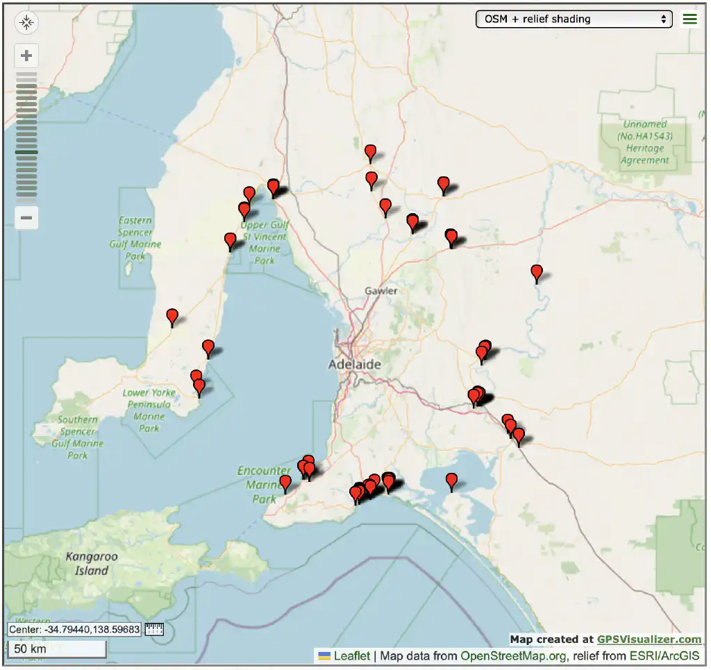
As expected, because of the distance restriction, we end up with a rough “ring” around Adelaide of places we can go eat.
Let’s try something different - what’s the furthest I could go for a bite to eat, without leaving my home state?
WITH boundary AS (
    SELECT
        ST_BuildArea (ST_Union (boundaries.geom)) AS geom
    FROM
        boundaries
    WHERE
        relation_id = 2316596
),
input_point AS (
    SELECT
        ST_Transform (ST_SetSRID (ST_MakePoint (138.6, -34.9), 4326), 3857) AS geom
)
SELECT
    ST_Distance (points.geom, input_point.geom)::INT AS dist,
    points.tags ->> 'name' AS name,
    ST_Y (ST_Transform (points.geom, 4326)) AS latitude,
    ST_X (ST_Transform (points.geom, 4326)) AS longitude
FROM
    points,
    input_point,
    boundary
WHERE
    ST_Within (points.geom, boundary.geom)
    AND tags ->> 'amenity' IN ('restaurant', 'pub', 'fast_food', 'bar', 'cafe')
ORDER BY
    dist DESC
LIMIT 70
We’re doing something a bit different here. We have a new addition to the CTE
definition, the boundary. We are selecting from the boundaries table which
contains OSM relations. We’ve
selected a single relation via id 2316596 which is the boundary of South
Australia.
The ST_BuildArea(ST_Union(boundaries.geom)) is necessary to turn the
geometry(MultiLineString,3857) data into an actual area we can compare to our
points. The geom column by itself in the boundaries table only describes a
series of lines, not an actual area polygon.
The rest is pretty straightforward, the WHERE clause uses the ST_Within PostGIS function to ensure the selected point is within the state, and that it is a place we can eat at.
The ORDER BY and LIMIT clauses gives us the furthest 70 ones in that set.
Running the query gives us:
┌─────────┬────────────────────────────────────┬─────────────────────┬────────────────────┐
│  dist   │                name                │      latitude       │     longitude      │
├─────────┼────────────────────────────────────┼─────────────────────┼────────────────────┤
│ 1153188 │                                    │ -31.638423399379143 │        129.0036768 │
│ 1153176 │                                    │ -31.638399599379145 │         129.003804 │
│ 1133415 │ Marla Bar                          │ -27.304119499479423 │        133.6231117 │
│  972694 │ Nullarbor Roadhouse                │ -31.449961599365615 │        130.8960597 │
│  972662 │ Nullarbor Roadhouse                │ -31.449953899365607 │         130.896391 │
│  884025 │ Opal Cafe                          │ -29.009138799345084 │ 134.75491339999996 │
│  883948 │ Mediterranean Street Food Tavern   │ -29.009393399345072 │        134.7558219 │
│  883934 │ Outback Restaurant                 │  -29.00952839934507 │        134.7557879 │
│  883821 │ Chicken                            │  -29.01073389934501 │        134.7554042 │
│  883819 │ Fish n Chips                       │  -29.01076669934501 │        134.7553774 │
│  883817 │ John's Pizza Coffee Lounge         │  -29.01076669934501 │        134.7554122 │
│  883659 │ Tom & Mary's Greek Taverna         │ -29.012697499344913 │         134.754345 │
│  883621 │ Pizza, Pasta, Chicken Cafe         │   -29.0131169993449 │        134.7541838 │
│  883604 │ Desert Grill & Seafood             │ -29.013260099344897 │        134.7541999 │
...
(As you can see, some of the entries lack a ’name’ tag in OSM).
Using \copy again lets us produce another nice map:
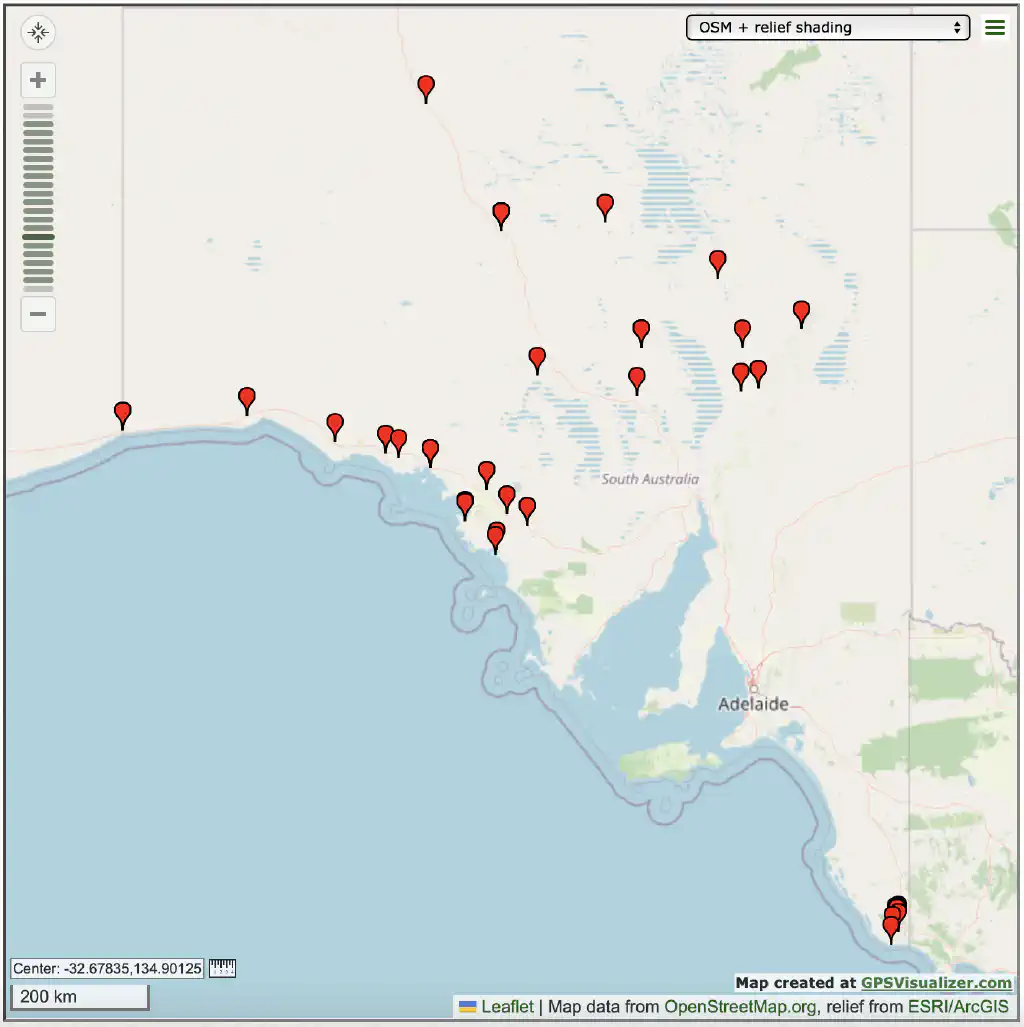
This map is quite interesting! The lack of places to eat in the north of the state is probably partly a reflection of just how little there is up there, and (I believe) partly a reflection of a lack of OSM activity up there. It is very remote, but it seems likely there are more places to eat that are simply not in the OSM database yet.
Tags: OSM PostgreSQL PostGIS GIS